
Notes about Datastream
This note reviews the article published years ago in Data stream research “Models and Issues in Data stream Systems“.
Section 2 The Data stream model
Differences between Data stream and Stored relational model
– Arrival : Data element in the stream arrives online
– Order control : There is no guarantee that data element comes in order and within the current processing stream.
– Unbounded size
– Not permanently stored in Memory: One a data element is processed, it then will be archived ( disk ?) or discarded. Hence, it will be no longer retrieved by accessing to Memory.
Section 3 Review of Data stream projects
Section 4 Queries over Data streams
This section addresses challenges of query processing in the data stream and solutions for them as well.
4.1 Unbounded Memory Requirements
The continuous queries require real-time response which cannot be fulfilled by traditional query processing algorithms. As data elements are generated at high rate over time, some of them come when the old data elements are being processed. Even if the computation time required for each data element is small, the old fashioned algorithm might still cannot handle the massive amount of upcoming data streams.
Arasu et al. wrote a paper [1] which concludes if the size of the input data streams, then it is not possible to limit the memory required for common queries including joins.
4.2 Approximate Query Answering
With queries over data streams, there is not always a precise answer. Therefore, a quality approximate answer is certainly a way to go.
Recent works touched upon several approaches to approximate answers mostly for correlated aggregate queries but not general queries.
4.3 Sliding Windows
One technique toward approximate answers is concerning the recent data but not over the past history of data streams. Data elements are processed within a range so called a window. That window slides as time goes by. The term sliding window is coined from that phenomenon. The question is how to form a window. Basically, the solution is equipping a data element with a timestamp which can be either the arrival time of the data element or explicit timestamp assigned by the data stream generator. The fundamental issue is how we define timestamps over the stream to facilitate the use of windows.
The implementation of sliding window queries and their impact on query optimization is a largely untouched area.
4.4 Batch Processing, Sampling, and Synopses
Batch processing
Sampling
Synopsis Data structures
4.5 Blocking Operators
A blocking query operator is query operator that cannot compute the result until the entire input data have arrived. For example : SUM, COUTN, MIN, MAX, and AVG. The blocking operator having a data stream as its inputs never sees its entire input, and therefore it will never be able to produce any output.
Note that, a query plan is actually a tree of query operators. If there are other query operators consuming the results of blocking operators which will be modified as a new data element arrives (as blocking query operators compute the result by processing the entire input, the input expands causing these operators to recompute).
One solution is replacing blocking operator with a non blocking operator. For instance: a non blocking version of sort operator. However, the question is to which extend we can substitute other blocking operators with their non blocking versions.
Another option is to augment data streams with assertions which are called as punctuations which are requirements for data elements in infinite data streams. They merely help to get rid of data elements which do not satisfy the condition. For example, “for all tuples, daynumber >= 10”, an aggregation operator that was grouping by daynumber could stream out its answers for all daynumbers less than 10.
Likely there is an idea of constrains on data streams (schema-level assertions) ( ????).
4.6 Queries Referencing Past Data
Ad hoc queries are queries which are installed and executed on the fly ( not predefined). One processing these queries, it makes troubles if some past data are needed to answer these queries. Why ? because we simply discarded the past data as data streams is expected to be infinite which one cannot accommodate all of them in the memory or even on disk
Section 5 Proposal for a DSMS
This section addresses challenges of query processing in the data stream and solutions for them as well.
This section primarily focuses on query language and query processing components of a DSMS.
5.1 Query language for a DSMS
The main modifications are made to standard SQL :
i) allowing the FROM clause to refer to streams as well as relations ii) is to extend the expressiveness of the query language for sliding windows.
The notion of sliding windows requires at least an ordering on data elements. Formally, a data stream S consists of a set of (tuple, timestamp) pairs {(s1, i1), (s2, i2), …, (sn, in)}. The timestamp attribute could be a traditional timestamp or it could be a sequence number.
So the window specification consists of : i ) an optional partitioning clause : how to partition data elements into several groups. ii) a window size : which can be a physical size ( number of data elements in a window) or logical size ( say, range of time covered by a window such as 7 days, a week) . iii) an optional filtering predicate.
Example 1 :
SELECT AVG(S.minutes)
FROM Calls S [PARTITION BY S.customer id
ROWS 10 PRECEDING
WHERE S.type = ’Long Distance’]
Example 2:
SELECT AVG(S.minutes)
FROM Calls S [PARTITION BY S.customer id
ROWS 10 PRECEDING]
WHERE S.type = ’Long Distance’
5.2 Timestamp in Streams
There are two types of timestamp ; Implicit timestamp and Explicit timestamp. The former is a special field to each incoming tuple added by the system. It is used when data element does not already include a timestamp attribue ( Why? Either the data source does not do it or it is not important for their own sakes to do so. But when it comes to our DSMS we need to judge its state as “recent” “old”). The latter ( explicit one ) is an attribute in data tuple assigned at its source. However, there is no grantee that data elements arrive in order as their timestamp. One associated with smaller timestamp can arrive later than another one with bigger timestamp. The sample problem raises when data elements expected come from different streams.
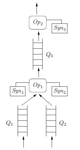
5.3 Query processing Architecture of a DSMS
Below is a sketch of a proposal for query processing architecture of a DSMS. Actually, this is a portion of a query plan in which Op1, Op2 . . . are query operators. In addition, Syn1, Syn2, and Syn3 are synopsis operators (together synopsis data structure ?? which are used for blocking operators ??? I guess). Besides, Q1, Q2 are buffers accommodating input streams.
Research questions:
– How difference a query operator produces approximation results under limited memory ? How differences given the same condition when query operators are composed as they appear in query plan.
– How can DSMS allocate memory to the operator to maximize the accuracy of the answer of the query . In other words, how wisely to allocate memory to minimize the approximation.
– Best memory allocation ( shared memory), minimize approximation ??
Reference
[1] A.Arasu, B. Babcock, S.Babu, J. McAlister, and J.Widom. Characterizing Memory Requirements for Queries over continuous data streams. In Proc. of the 2002 ACM Symp. on Principles of Database Systems, June 2002. Available at http://dbpubs.standford.edu/pub/2001-49. Continuous Data Streams